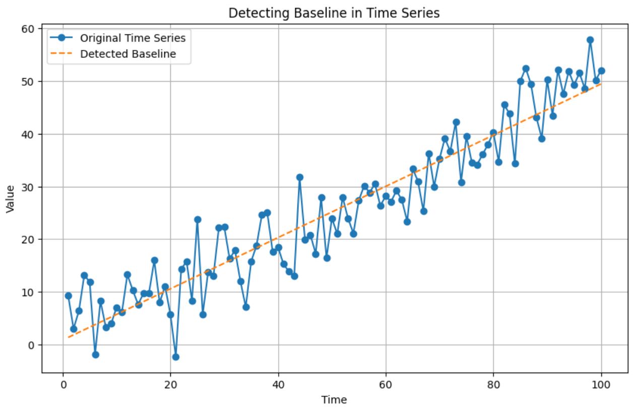
 If you’ve ever wrestled with forecasting time series data, you know that starting with a reliable baseline can make all the difference. In this piece, we pick up where we left off—exploring how to break down your data into trend, seasonality, and noise, and using those insights to build a more accurate baseline model.
Earlier, we applied a Seasonal Naive forecast to daily temperature data. While it nailed the broad seasonal trends, its Mean Absolute Percentage Error (MAPE) of 28.23% revealed it wasn’t quite capturing the subtle shifts and long-term movements in the data. The approach of predicting a value based purely on the same day in the previous year doesn’t always fit the bill when both trend and seasonality play a role. That’s why fine-tuning your baseline using a more tailored method can set a solid foundation before you dive into models like ARIMA.
In Part 1, we visualised trends and seasonality using Python’s seasonal_decompose function. Now, by processing a 14-day temperature sample manually, we can peel back the layers of this method:
Trend: We use a 3-day centred moving average to smooth daily fluctuations. For example, the trend on February 1, 1981, is calculated as (20.7 + 17.9 + 18.8) / 3 = 19.13°C. Because the moving average needs data on both sides, the first and last days remain without a trend value.
Seasonality: Once the trend is removed from the observed values, we’re left with a detrended series that accentuates seasonal patterns. Grouping these values by a weekly Day Index (1 through 7) allows us to average out the fluctuations—for instance, averaging detrended values from January 2 and January 9 gives us a good snapshot of that day’s seasonal effect.
What’s left is the residual, computed simply as Observed Value – Trend – Seasonality. Although early detrended values incorporate some noise, grouping by cycle helps isolate that consistent seasonal pulse. It’s normal to see missing residuals where trend values aren’t available.
After splitting your dataset into training and testing segments, you can apply these techniques to forecast future values. For the trend, extending the last observed training value across the test period, combined with the seasonal insights, delivers a baseline forecast that brings the MAPE down to 21.21%—a meaningful improvement over the initial model.
We then stepped up our approach by creating custom baselines. Averaging the temperature for each day of the year in the training data provided forecasts that hit a MAPE of 21.17%. Refining this further with a calendar-day method—and smoothing over leap year quirks—reduced the error slightly to 21.09%. A final blend, which gave 70% weight to calendar averages and 30% to the previous day’s temperature, pushed the MAPE down to an impressive 18.73%.
This practical, easy-to-understand process not only explains much of the variance in your data but also sets the stage for more advanced techniques. Whether you’re new to forecasting or looking to sharpen your models, these steps offer a clear path forward. In future posts, we’ll explore techniques like STL decomposition and more advanced models such as ARIMA and SARIMA, paving the way for robust multi-variable analysis.


